Un-replicated Optimized Arrangement Design
Source:vignettes/optimized_arrangement.Rmd
optimized_arrangement.RmdThis vignette shows how to generate an un-replicated
optimized arrangement design using both the FielDHub Shiny App
and the scripting function optimized_arrangement() from the
FielDHub R package.
Overview
One un-replicated design you can use in FielDHub is the optimized arrangement. Unlike the diagonal design, the optimized arrangement completely randomizes the positions for the checks instead of putting them in a systematic diagonal pattern(Clarke and Stefanova 2011). Randomization is subject to some restrictions. These restrictions seek to optimize the distribution of control plots in the field and ensure they are spread while keeping a minimum distance between them.
FielDHub includes a function to run such experimental
designs, features include options to set the number of entries and the
number of checks for the experiment. Users can also choose to run the
same experiment over multiple locations.
Use case
An early generation plant breeding project needs to test 401 genotypes of winter wheat. It is planned to carry out this experiment on a field containing 29 rows and 15 columns of plots. In this project, these 401 genotypes are allocated into one experiment and tested over three locations. In addition, three checks are randomly included across field to fill 34 plots representing 7.8% of the total number of experimental plots.
1. Using the FielDHub Shiny App
Once the app is running, go to un-replicated Designs > Optimized Arrangement
Then, follow the following steps where we will show how to generate an un-replicated optimized arrangement design.
Inputs
-
Import entries’ list? Choose whether to import a
list with entry numbers and names for genotypes or treatments.
If the selection is
No, that means the app is going to generate synthetic data for entries and names of the treatment/genotypes based on the user inputs.If the selection is
Yes, the entries list must fulfill a specific format and must be a.csvfile. The file must have the columnsENTRY,NAME, andREPS. TheENTRYcolumn must have a unique entry integer number for each treatment/genotype. The columnNAMEmust have a unique name that identifies each treatment/genotype. TheREPScolumn must have an integer entry for the replications of the checks and other entries. Both ENTRY and NAME must be unique, duplicates are not allowed. In the following table, we show an example of the entries list format. This example has an entry list with three checks and nine treatments/genotypes. It is crucial to allocate the checks in the top part of the file.
| ENTRY | NAME | REPS |
|---|---|---|
| 1 | CHECK1 | 10 |
| 2 | CHECK2 | 10 |
| 3 | CHECK3 | 10 |
| 4 | G-4 | 1 |
| 5 | G-5 | 1 |
| 6 | G-6 | 1 |
| 7 | G-7 | 1 |
| 8 | G-8 | 1 |
| 9 | G-9 | 1 |
| 10 | G-10 | 1 |
| 11 | G-11 | 1 |
| 12 | G-12 | 1 |
Enter the number of checks in the Input # of Checks box, which is
3in our case.Enter the number of replications of the checks in a comma separated list containing a number for each check in the Input # Check’s Reps box. For our example experiment, we will enter
12,11,11.Enter the number of entries/treatments in the Input # of Entries box, which is
401in our case.Select
serpentineorcartesianin the Plot Order Layout. For this example we will set theserpentinelayout.Since we want to run this experiment over 3 locations, set Input # of Locations to
3.To ensure that randomizations are consistent across sessions, we can set a random seed in the box labeled random seed. For instance, we will set it to
130.Enter the name for the experiment in the Input Experiment Name box. For example,
PYT_WHEAT_22.Enter the starting plot number in the Starting Plot Number box. If the experiment has multiple locations, you must enter a comma separated list of numbers the length of the number of locations for the input to be valid. Since we have 3 locations in this experiment, we will enter
1001,2001,3001.Enter the name of the site/location in the Input the Location box. In our case we will run the experiment in three locations, the name for each location must be enter separate by comma, for example:
FARGO, CASSELTON, MINOT.Once we have entered the information for our experiment on the left side panel, click the Run! button to run the design.
You will then be prompted to select the dimensions of the field from the list of options in the drop down in the middle of the screen with the box labeled Select dimensions of field. In our case, we will select
15 x 29.Click the Randomize! button to randomize the experiment with the set field dimensions and to see the output plots. If you change the dimensions again, you must re-randomize.
If you change any of the inputs on the left side panel after running an experiment initially, you have to click the Run and Randomize buttons again, to re-run with the new inputs.
Outputs
After you run an un-replicated optimized arrangement design in FielDHub and set the dimensions of the field, there are several ways to display the information contained in the field book. The first tab, Get Random, shows the option to change the dimensions of the field and re-randomize, as well as a reference guide for experiment design.
Data Input
On the second tab, Data Input, you can see all the entries in the randomization in a list, as well as a table of the checks with the number of times they appear in the field. In the list of entries, the reps for each check is included as well.
Randomized Field
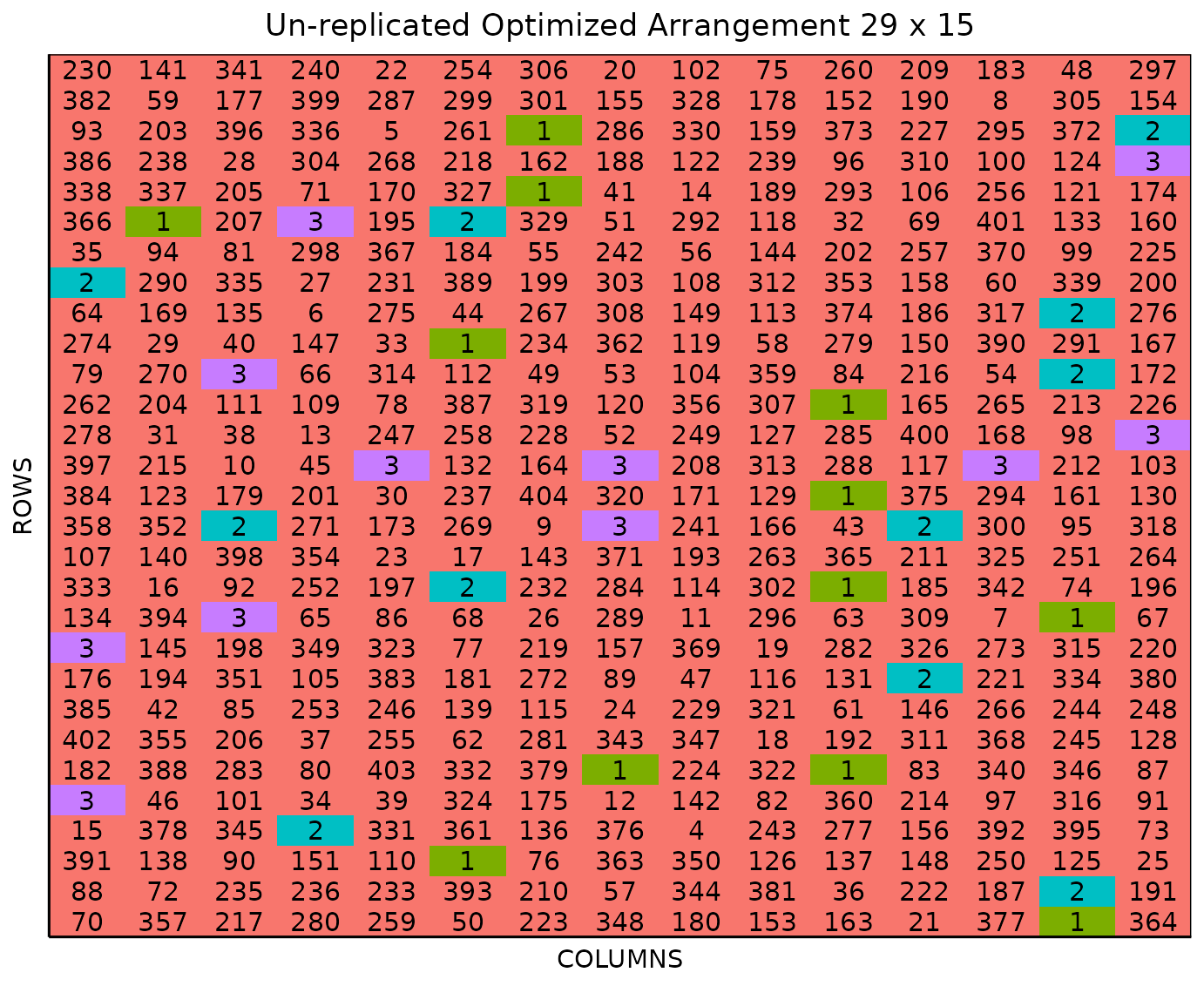
The Randomized Field tab displays a graphical representation of the randomization of the entries in a field of the specified dimensions. The checks are all colored uniquely, showing the number of times they are distributed throughout the field. The display includes numbered labels for the rows and columns. You can copy the field as a table or save it directly as an Excel file with the Copy and Excel buttons at the top.
Plot Number Field
On the Plot Number Field tab, there is a table display of the field with the plots numbered according to the Plot Order Layout specified, either serpentine or cartesian. You can see the corresponding entries for each plot number in the field book. Like the Randomized Field tab, you can copy the table or save it as an Excel file with the Copy and Excel buttons.
Field Book
The Field Book displays all the information on the
experimental design in a table format. It contains the specific plot
number and the row and column address of each entry, as well as the
corresponding treatment on that plot. This table is searchable, and we
can filter the data in relevant columns.
2. Using the FielDHub function:
optimized_arrangement().
You can run the same design with the function
optimized_arrangement() in the FielDHub
package.
First, you need to load the FielDHub package typing,
Then, you can enter the information describing the above design like this:
optim_expt <- optimized_arrangement(
  nrows = 29,
  ncols = 15,
  lines = 401,
  amountChecks = c(12,11,11),
  checks = 3,
  l = 3,
  plotNumber = c(1001,2001,3001),
  exptName = "WINTER_WHEAT_22",
  locationNames = c("FARGO", "CASSELTON", "MINOT"),
  seed = 130
)
Details on the inputs entered in
optimized_arrangement() above
The description for the inputs that we used to generate the design,
-
nrows = 29is the number of rows in the field. -
ncols = 15is the number of columns in the field. -
lines = 401is the number of entries -
amountChecks = c(12,11,11)are the values for representing respective replicates of each check, or an integer total number of checks. -
checks = 3is the number of checks. -
l = 3is the number of locations. -
plotNumber = c(1001,2001,3001)are the starting plot number for each location respectively, or a single number for 1 location. -
exptName = "WINTER_WHEAT_22"is an optional name for experiment. -
locationNames = c("FARGO", "CASSELTON", "MINOT")are the values for representing respective name for each location. -
seed = 130is the random seed to replicate identical randomizations.
Print optim_expt object
To print a summary of the information that is in the object
optim_expt, we can use the generic function
print().
print(optim_expt)Un-replicated Optimized Arrangement Design
Information on the design parameters:
List of 10
$ rows : num 29
$ columns : num 15
$ min_distance: num [1:3] 1.41 1 1
$ treatments : num 401
$ checks : int 3
$ entry_checks: int [1:3] 1 2 3
$ rep_checks : num [1:3] 12 11 11
$ locations : num 3
$ planter : chr "serpentine"
$ seed : num 130
10 First observations of the data frame with the optimized_arrangement field book:
ID EXPT LOCATION YEAR PLOT ROW COLUMN CHECKS ENTRY TREATMENT
1 1 WINTER_WHEAT_22 FARGO 2026 1001 1 1 0 98 G98
2 2 WINTER_WHEAT_22 FARGO 2026 1002 1 2 0 190 G190
3 3 WINTER_WHEAT_22 FARGO 2026 1003 1 3 0 4 G4
4 4 WINTER_WHEAT_22 FARGO 2026 1004 1 4 0 341 G341
5 5 WINTER_WHEAT_22 FARGO 2026 1005 1 5 0 286 G286
6 6 WINTER_WHEAT_22 FARGO 2026 1006 1 6 0 7 G7
7 7 WINTER_WHEAT_22 FARGO 2026 1007 1 7 0 114 G114
8 8 WINTER_WHEAT_22 FARGO 2026 1008 1 8 0 185 G185
9 9 WINTER_WHEAT_22 FARGO 2026 1009 1 9 0 283 G283
10 10 WINTER_WHEAT_22 FARGO 2026 1010 1 10 0 218 G218Access to optim_expt object
The optimized_arrangement() function returns a list
consisting of all the information displayed in the output tabs in the
FielDHub app: design information, plot layout, plot numbering, entries
list, and field book. These are Accessible by the $
operator, i.e. optim_expt$layoutRandom or
optim_expt$fieldBook.
optim_expt$fieldBook is a data frame containing
information about every plot in the field, with information about the
location of the plot and the treatment in each plot. As seen in the
output below, the field book has columns for ID,
EXPT, LOCATION, YEAR,
PLOT, ROW, COLUMN,
CHECKS, ENTRY, and TREATMENT.
Let us see the first 10 rows of the field book for this experiment.
field_book <- optim_expt$fieldBook
head(field_book, 10)
ID EXPT LOCATION YEAR PLOT ROW COLUMN CHECKS ENTRY TREATMENT
1 1 WINTER_WHEAT_22 FARGO 2026 1001 1 1 0 98 G98
2 2 WINTER_WHEAT_22 FARGO 2026 1002 1 2 0 190 G190
3 3 WINTER_WHEAT_22 FARGO 2026 1003 1 3 0 4 G4
4 4 WINTER_WHEAT_22 FARGO 2026 1004 1 4 0 341 G341
5 5 WINTER_WHEAT_22 FARGO 2026 1005 1 5 0 286 G286
6 6 WINTER_WHEAT_22 FARGO 2026 1006 1 6 0 7 G7
7 7 WINTER_WHEAT_22 FARGO 2026 1007 1 7 0 114 G114
8 8 WINTER_WHEAT_22 FARGO 2026 1008 1 8 0 185 G185
9 9 WINTER_WHEAT_22 FARGO 2026 1009 1 9 0 283 G283
10 10 WINTER_WHEAT_22 FARGO 2026 1010 1 10 0 218 G218Plot the field layout
For plotting the layout in function of the coordinates
ROW and COLUMN in the field book object we can
use the generic function plot() as follow,
plot(optim_expt)
The figure above shows a map of an experiment randomized as an un-replicated optimized arrangement design. Gray plots represent the un-replicated treatments, while distinctively colored check plots are randomly replicated throughout the field.
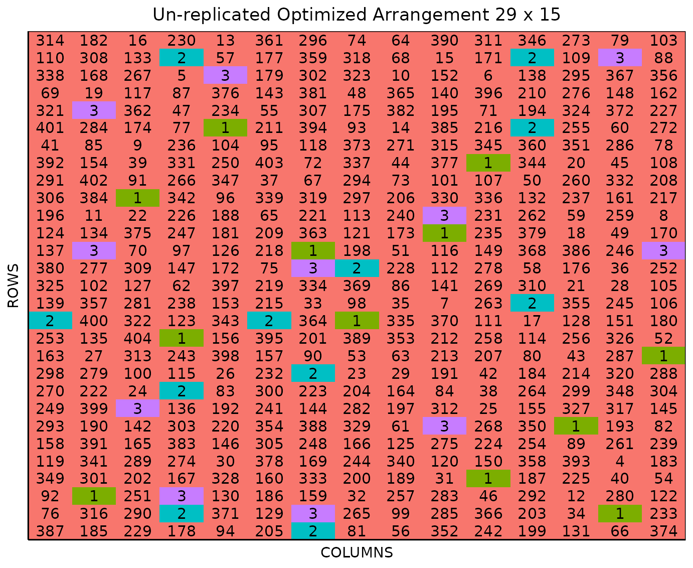
It is possible to pass more arguments to plot() such as
the specific location. For example, you can plot specifically the layout
for location 2.
plot(optim_expt, l = 2)