Partially Replicated (p-rep) Design
Source:vignettes/partially_replicated.Rmd
partially_replicated.RmdThis vignette shows how to generate a partially replicated
(p-rep) design using both the FielDHub Shiny App and the
scripting function partially_replicated() from the
FielDHub R package.
Overview
Partially replicated designs are commonly employed in early generation field trials. This type of design is characterized by replication of a portion of the entries, with the remaining entries only appearing once in the experiment. Commonly, the part of treatments with reps is due to an arbitrary decision by the research, also in some cases, it is due to technical reasons. The replication ratio is typically 1:4 (Cullis 2006), which means that the portion of treatment repeated twice is p = 25%. However, the design can be adapted to meet specific needs by adjusting the values of and the level of replication. For example, standard varieties (checks) may be included with higher levels of replication than test lines.
In FielDHub, users can set the number of entries that
will have reps, as well as the number of entries that will only appear
once. You can also choose to run the same experiment over multiple
locations.
Optimization
Each partially replicated (p-rep) design location undergoes an optimization process that involves the following procedure:
Given a matrix of integers (p-rep design within location), we want to ensure that the distance between any two occurrences of the same treatment is at least a distance . More specifically, we want to modify to ensure that no treatments appear twice within a distance less than in the resulting matrix.
The goal of the optimization process is to find a modified matrix
that satisfies this constraint while maximizing some measure of
deviation from the original matrix
.
In this case, the measure of deviation is the pairwise Euclidean
distance between occurrences of the same treatment. The process is done
by the function swap_pairs() that uses a heuristic
algorithm that starts with a distance of
between pairs of occurrences of the same treatment, and increases this
distance by
and repeats the process until either the algorithm no longer converges
or the maximum number of iterations is reached.
The algorithm works by first identifying all pairs of occurrences of the same treatment that are closer than . For each such pair, the function selects a random occurrence of a different integer that is at least away, and swaps the two occurrences. This process is repeated until no further swaps can be made that increase the pairwise Euclidean distances between occurrences of the same treatment.
Toy Example
Consider a p-rep design where ten treatments are replicated twice and forty only once. The matrix (field layout) for this experiment has 6 rows and 10 columns.
     [,1] [,2] [,3] [,4] [,5] [,6] [,7] [,8] [,9] [,10]
[1,]   21   40   17   25   26    3   11   31   36     6
[2,]    5    5   33    8   48   29   43   23    1    45
[3,]   41   27   38   39    7   28   14   22   24     4
[4,]    4   47   18    7    2   35    6   20   12    46
[5,]    3   15    9   34   49   50    2   10   42     8
[6,]   32   16   19    9   10   13   37    1   44    30
In this initial p-rep design, we notice that the two instances of treatment 5 are positioned next to each other. Additionally, treatments 7 and 9 are also situated in adjacent cells. These suboptimal allocations could lead to issues or inaccurate results when analyzing the data from this experiment due to the short distance between replicated treatments and the likely spatial correlation between them.
The following table shows the pairwise distances for the replicated treatments
   geno Pos1 Pos2     DIST rA cA rB cB
1     5    2    8 1.000000  2  1  2  2
2     7   22   27 1.414214  4  4  3  5
3     9   17   24 1.414214  5  3  6  4
4     2   28   41 2.236068  4  5  5  7
5    10   30   47 3.162278  6  5  5  8
6     1   48   50 4.123106  6  8  2  9
7     6   40   55 4.242641  4  7  1 10
8     3    5   31 6.403124  5  1  1  6
9     8   20   59 6.708204  2  4  5 10
10    4    4   57 9.055385  4  1  3 10
Swap pairs
We can improve the efficiency of the design by swapping the
treatments that are close and next to each other by using the function
swap_pairs() from FielDHub R package.
library(FielDHub)
B <- swap_pairs(X, starting_dist = 3)
The new matrix or the optimized p-rep design is,
print(B$optim_design)
     [,1] [,2] [,3] [,4] [,5] [,6] [,7] [,8] [,9] [,10]
[1,]   21   40   17    2    5    3   11   31   36     6
[2,]    8   43   33   34   48   29    7   23    1    45
[3,]   41   27    9   39   10   28   14    9   24     4
[4,]    4   47   18   26   25   35    6   20   12    46
[5,]    3   15   22    2   49   50    5    7   42     8
[6,]   32   16   19   38   10   13   37    1   44    30
The distances for each pairwise of treatments are,
print(B$pairwise_distance)
   geno Pos1 Pos2     DIST rA cA rB cB
1    10   27   30 3.000000  3  5  6  5
2     7   38   47 3.162278  2  7  5  8
3     2   19   23 4.000000  1  4  5  4
4     1   48   50 4.123106  6  8  2  9
5     6   40   55 4.242641  4  7  1 10
6     5   25   41 4.472136  1  5  5  7
7     9   15   45 5.000000  3  3  3  8
8     3    5   31 6.403124  5  1  1  6
9     4    4   57 9.055385  4  1  3 10
10    8    2   59 9.486833  2  1  5 10
As we can see, the minimum distance that the algorithm reached is 3. This means no treatments appear twice within a distance less than 3 in the resulting prep design. It is a considerable improvement from the first version of the p-rep design
The FielDHub function
partially_replicated() does internally all the optimization
process and uses the function swap_pairs() to maximize the
distance between replicated treatments.
Acknowledge
We would like to acknowledge Mr. Jean-Marc Montpetit for contributing
code and ideas for the swap_pairs() and
pairs_distance() functions. His contributions have had a
significant impact on improving the partially replicated (p-rep) design
in the R package FielDHub. We thank him for his valuable
contributions.
Use case
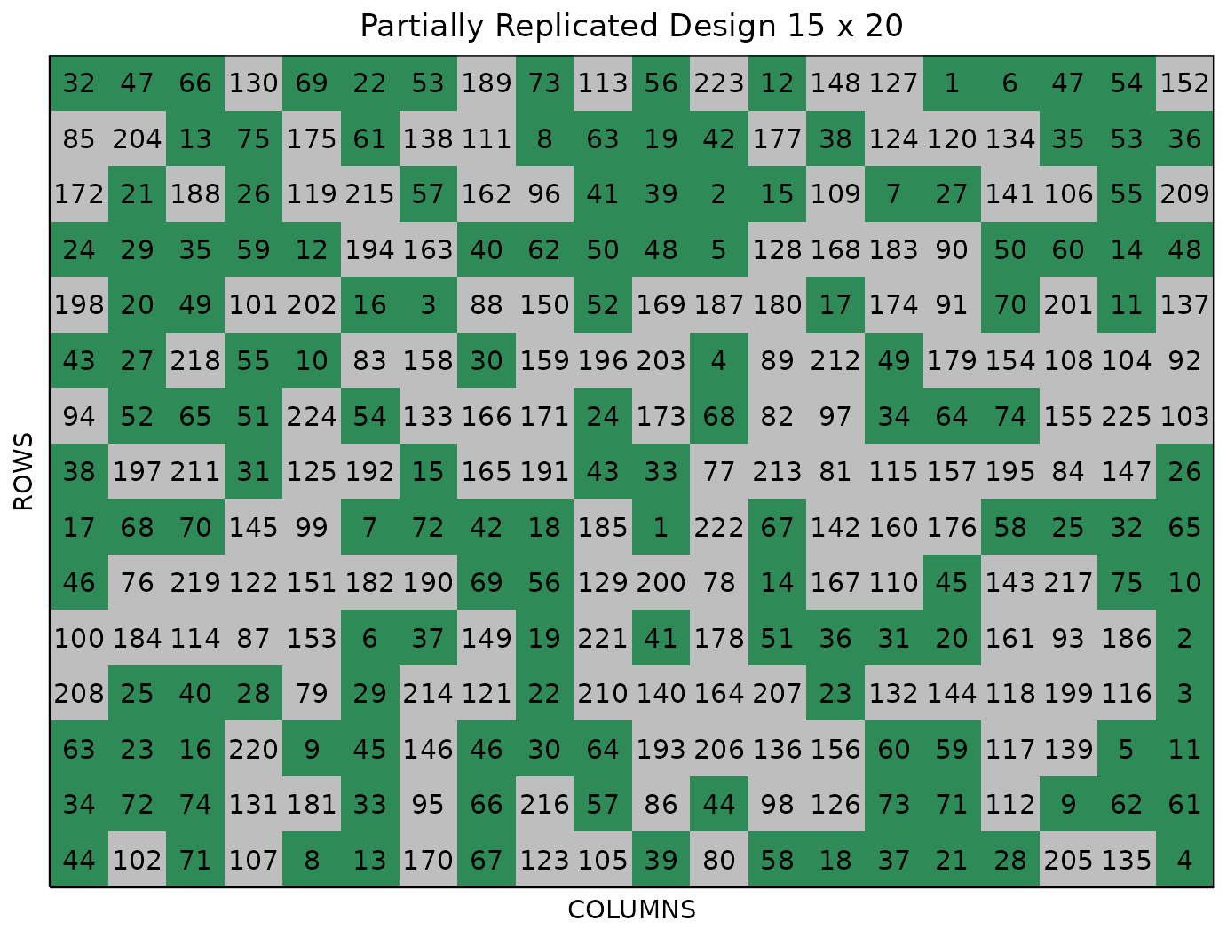
Consider a plant breeding field trial with 300 plots containing 75 entries appearing two times each, and 150 entries only appearing once. This field trial is arranged in a field of 15 rows by 20 columns. In this case, the breeder decided to replicate the genotypes that do not share significant generic information with each other (75), as well as leave with just one copy the genotypes that are siblings (150).
1. Using the FielDHub Shiny App
Once the app is running, click the tab Partially Replicated Design and select Single and Multi-Location p-rep from the dropdown.
Then, follow the following steps where we will show how to generate a partially replicated design.
Inputs
-
Import entries’ list? Choose whether to import a
list with entry numbers and names for genotypes or treatments.
If the selection is
No, that means the app is going to generate synthetic data for entries and names of the treatment/genotypes based on the user inputs.If the selection is
Yes, the entries list must fulfill a specific format and must be a.csvfile. The file must have the columnsENTRY,NAME, andREPS. TheENTRYcolumn must have a unique entry integer number for each treatment/genotype. The columnNAMEmust have a unique name that identifies each treatment/genotype. TheREPScolumn must have an integer number for the replications of the groups. Both ENTRY and NAME must be unique, duplicates are not allowed. In the following table, we show an example of the entries list format. This example has an entry list with four treatments/genotypes that will appear twice and 8 that appear just once.
| ENTRY | NAME | REPS |
|---|---|---|
| 1 | GenotypeA | 2 |
| 2 | GenotypeB | 2 |
| 3 | GenotypeC | 2 |
| 4 | GenotypeD | 2 |
| 5 | GenotypeE | 1 |
| 6 | GenotypeF | 1 |
| 7 | GenotypeG | 1 |
| 8 | GenotypeH | 1 |
| 9 | GenotypeI | 1 |
| 10 | GenotypeJ | 1 |
| 11 | GenotypeK | 1 |
| 12 | GenotypeL | 1 |
Enter the number of entries per replicate group in the # of Entries per Rep Group box as a comma separated list. In our example we will have 2 groups with 85 and 130 entries. So, we enter
75, 150in the box for our sample experiment.Enter the number of replications per group in the # of Rep per Group box. In our example we will have 2 and 1 replications for the 2 groups, so we enter
2, 1in this box.Enter the number of locations in Input # of Locations. We will run this experiment over a single location, so set Input # of Locations to
1.Select
serpentineorcartesianin the Plot Order Layout. For this example we will use the defaultserpentinelayout.To ensure that randomizations are consistent across sessions, we can set a random seed in the box labeled random seed. In this example, we will set it to
1245.Enter the starting plot number in the Starting Plot Number box. If the experiment has multiple locations, you must enter a comma separated list of numbers the length of the number of locations for the input to be valid.
Once we have entered the information for our experiment on the left side panel, click the Run! button to run the design.
You will then be prompted to select the dimensions of the field from the list of options in the drop down in the middle of the screen with the box labeled Select dimensions of field. In our case, we will select
15 x 20.Click the Randomize! button to randomize the experiment with the set field dimensions and to see the output plots. If you change the dimensions again, you must re-randomize.
If you change any of the inputs on the left side panel after running an experiment initially, you have to click the Run and Randomize buttons again, to re-run with the new inputs.
Outputs
After you run a single diagonal arrangement in FielDHub and set the dimensions of the field, there are several ways to display the information contained in the field book. The first tab, Get Random, shows the option to change the dimensions of the field and re-randomize, as well as a reference guide for experiment design.
Data Input
On the second tab, Data Input, you can see all the entries in the randomization in a list, as well as a table of the checks with the number of times they appear in the field. In the list of entries, the reps for each check is included as well.
Randomized Field
The Randomized Field tab displays a graphical representation of the randomization of the entries in a field of the specified dimensions. The checks are the green colored cells, with the The display includes numbered labels for the rows and columns. You can copy the field as a table or save it directly as an Excel file with the Copy and Excel buttons at the top.
Plot Number Field
On the Plot Number Field tab, there is a table display of the field with the plots numbered according to the Plot Order Layout specified, either serpentine or cartesian. You can see the corresponding entries for each plot number in the field book. Like the Randomized Field tab, you can copy the table or save it as an Excel file with the Copy and Excel buttons.
Field Book
The Field Book displays all the information on the experimental design in a table format. It contains the specific plot number and the row and column address of each entry, as well as the corresponding treatment on that plot. This table is searchable, and we can filter the data in relevant columns.
2. Using the FielDHub function:
partially_replicated().
You can run the same design with the function
partially_replicated() in the FielDHub
package.
First, you need to load the FielDHub package typing,
Then, you can enter the information describing the above design like this:
prep <- partially_replicated(
  nrows = 15,
  ncols = 20,
  repGens = c(75,150),
  repUnits = c(2,1),
  planter = "serpentine",
  plotNumber = 101,
  l = 1,
  exptName = "Expt1",
  locationNames = "PALMIRA",
  seed = 1245,
)
Details on the inputs entered in
optimized_arrangement() above
The description for the inputs that we used to generate the design,
-
nrows = 15is the number of rows in the field. -
ncols = 20is the number of columns in the field. -
repGens = c(75,150)are the values for the groups to replicate -
repUnits = c(2,1)are the values for representing respective replicates of each group. -
planter = "serpentine"is the layout order. -
plotNumber = 101is the starting plot number for the experiment. -
l = 1is the number of locations. -
exptName = "Expt1"is an optional name for experiment. -
locationNames = "PALMIRA"is the optional name for the locations. -
seed = 1245is the random seed to replicate identical randomizations.
Print prep object
To print a summary of the information that is in the object
prep, we can use the generic function
print().
print(prep)Partially Replicated Design
Replications within location:
LOCATION Replicated Unreplicated
1 PALMIRA 75 150
Information on the design parameters:
List of 7
$ rows : num 15
$ columns : num 20
$ min_distance : num 5
$ incidence_in_rows: num 4
$ locations : num 1
$ planter : chr "serpentine"
$ seed : num 1245
10 First observations of the data frame with the partially_replicated field book:
[38;5;246m# A tibble: 10 × 11
[39m
ID EXPT LOCATION YEAR PLOT ROW COLUMN REP CHECKS ENTRY TREATMENT
[3m
[38;5;246m<int>
[39m
[23m
[3m
[38;5;246m<chr>
[39m
[23m
[3m
[38;5;246m<chr>
[39m
[23m
[3m
[38;5;246m<chr>
[39m
[23m
[3m
[38;5;246m<dbl>
[39m
[23m
[3m
[38;5;246m<int>
[39m
[23m
[3m
[38;5;246m<int>
[39m
[23m
[3m
[38;5;246m<int>
[39m
[23m
[3m
[38;5;246m<dbl>
[39m
[23m
[3m
[38;5;246m<dbl>
[39m
[23m
[3m
[38;5;246m<chr>
[39m
[23m
[38;5;250m 1
[39m 1 Expt1 PALMIRA 2026 101 1 1 1 0 206 G206
[38;5;250m 2
[39m 2 Expt1 PALMIRA 2026 102 1 2 1 0 162 G162
[38;5;250m 3
[39m 3 Expt1 PALMIRA 2026 103 1 3 1 67 67 G67
[38;5;250m 4
[39m 4 Expt1 PALMIRA 2026 104 1 4 1 0 95 G95
[38;5;250m 5
[39m 5 Expt1 PALMIRA 2026 105 1 5 1 17 17 G17
[38;5;250m 6
[39m 6 Expt1 PALMIRA 2026 106 1 6 1 0 109 G109
[38;5;250m 7
[39m 7 Expt1 PALMIRA 2026 107 1 7 1 0 94 G94
[38;5;250m 8
[39m 8 Expt1 PALMIRA 2026 108 1 8 1 33 33 G33
[38;5;250m 9
[39m 9 Expt1 PALMIRA 2026 109 1 9 1 38 38 G38
[38;5;250m10
[39m 10 Expt1 PALMIRA 2026 110 1 10 1 16 16 G16 Access to prep output
The partially_replicated() function returns a list
consisting of all the information displayed in the output tabs in the
FielDHub app: design information, plot layout, plot numbering, entries
list, and field book. These are Accessible by the $
operator, i.e. prep$layoutRandom or
prep$fieldBook.
prep$fieldBook is a list containing information about
every plot in the field, with information about the location of the plot
and the treatment in each plot. As seen in the output below, the field
book has columns for ID, EXPT,
LOCATION, YEAR, PLOT,
ROW, COLUMN, CHECKS,
ENTRY, and TREATMENT.
Let us see the first 10 rows of the field book for this experiment.
field_book <- prep$fieldBook
head(field_book, 10)
[38;5;246m# A tibble: 10 × 11
[39m
      ID EXPT  LOCATION YEAR   PLOT   ROW COLUMN   REP CHECKS ENTRY TREATMENT

[3m
[38;5;246m<int>
[39m
[23m
[3m
[38;5;246m<chr>
[39m
[23m
[3m
[38;5;246m<chr>
[39m
[23m
[3m
[38;5;246m<chr>
[39m
[23m
[3m
[38;5;246m<dbl>
[39m
[23m
[3m
[38;5;246m<int>
[39m
[23m
[3m
[38;5;246m<int>
[39m
[23m
[3m
[38;5;246m<int>
[39m
[23m
[3m
[38;5;246m<dbl>
[39m
[23m
[3m
[38;5;246m<dbl>
[39m
[23m
[3m
[38;5;246m<chr>
[39m
[23m

[38;5;250m 1
[39m     1 Expt1 PALMIRA  2026    101     1      1     1      0   206 G206

[38;5;250m 2
[39m     2 Expt1 PALMIRA  2026    102     1      2     1      0   162 G162

[38;5;250m 3
[39m     3 Expt1 PALMIRA  2026    103     1      3     1     67    67 G67

[38;5;250m 4
[39m     4 Expt1 PALMIRA  2026    104     1      4     1      0    95 G95

[38;5;250m 5
[39m     5 Expt1 PALMIRA  2026    105     1      5     1     17    17 G17

[38;5;250m 6
[39m     6 Expt1 PALMIRA  2026    106     1      6     1      0   109 G109

[38;5;250m 7
[39m     7 Expt1 PALMIRA  2026    107     1      7     1      0    94 G94

[38;5;250m 8
[39m     8 Expt1 PALMIRA  2026    108     1      8     1     33    33 G33

[38;5;250m 9
[39m     9 Expt1 PALMIRA  2026    109     1      9     1     38    38 G38

[38;5;250m10
[39m    10 Expt1 PALMIRA  2026    110     1     10     1     16    16 G16